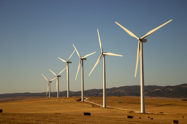
Wind Power Generation

Introduction
Utilizing renewable energy sources has become a global trend, as countries around the world
have rapidly increased their share of renewable energy supplies such as solar, wind, tides
and waves, geothermal heat, etc. While renewable sources are clean and
environmental-friendly compared to traditional sources, sun and wind energy depend on the
weather and can be unstable energy supplies. Therefore, it is important to predict such
energy output in a timely and accurate way to ensure optimal supply and demand planning in
an electric grid. The goal of this study is to investigate output from wind turbines. Wind
energy is generated by the mechanical power of wind on turbines that generate electricity.
This makes wind energy very sensitive to weather factors such as wind speed. Machine
learning (ML) techniques play a vital role in addressing this problem, where weather records
are available. Here we apply SpeedWise® Machine Learning (a commercial AutoML solution) to
generate a prediction of wind energy production.
Problem Description, Solution and Machine Learning Results
Problem Description
This dataset has been gathered from a wind turbine over a one year period, at 10-minute
intervals. The dataset includes power generation data and weather records. Our goal here
is to accurately model the power generation of the turbine based off the measured
parameters observed from the weather records. For that we used SpeedWise Machine
Learning (SML), which is a powerful AutoML solution that can automatically deal with the
idiosyncrasy of real data (the one considered here is a large, incomplete and noisy
dataset) while being able to automatically extract patterns, trends and correlations
from this data.
What was I looking to accomplish with machine learning?
The idea is to build a model that can automatically identify the relationship between
wind power generation and a set of records data (time, wind speed, wind direction,
etc.). Therefore, our target in this case will be the wind power generation. The power
generation represents continuous values, which can be described by solving a regression
problem. Once an optimum machine learning model is identified, we will review and
evaluate the metrices related to our regression problem to understand the ability of our
model to predict power generation. Our assumption is that the meteorological inputs are
given and can be used to generate the prediction.
Unwrapping the Data
The dataset for this study includes a total of 58,415 entries and 13 features or
attributes associated with each entry. This means the dataset is a table with more than
880,156 cells. Figure 1 shows the different measurement points from our wind turbine.
The meteorological measurements consist of date and time record for each observation.
The system records include temperature measurements of different parts, nacelle
position, rotor data etc. This information can be used to identify faulty or
suboptimally performing equipment. The generation data consists of a record the amount
of power generated by the turbine (units – kW). Observations are recorded at 15-minute
intervals.
 Figure 1: Wind energy diagram.
Data preprocessing is an essential step in building a robust and meaningful machine learning
model. SML allows users to cleanse their data efficiently, systematically and quickly. For
this dataset, our first step is to convert the time and date parameters into a more useful
format. Next, we take care of the missing data using SML’s automatic imputation step.
Alternatively, users can remove data by column or by row, which are also operations
available in SML. In this problem the system records should be remove since it won’t be
available when new prediction is generated. In fact, the system records can be used as a
target in a different machine learning problem to predict the failure of a particular part.
To get a better understanding of the data, several variables were visualized using the
Visualization function in SML.
 Figure 2: Visualization of the data in the procesing step
The plots in Figure 2 show that wind speed has a strong correlation with energy generation.
It’s also observed that there is no improvement in the power generation when wind speed >
7.5 mi/hr. No clear trend is observed between energy generation and wind direction. The data
also shows that the nacelle position follows the wind direction suggesting good performances
of the wind tracker. To further help visualize any relationships between the variables, a
Pearson correlation heatmap was plotted. The Pearson correlation plot shows a positive
correlation between power generation wind speed, direction and time of the day.
 Figure 3: Pearson correlation of the data
Results
SpeedWise Machine Learning was able to generate good machine learning models for the problem
at hand in a matter of minutes. In this case, the technology found a model (XGBoost) that
explains 97% of the variation in wind power generation. Some key metrics from the actual
model performance are shown in Figure 4. The Ground Truth vs. Prediction plot is shown to
evaluate the accuracy of the model. The gray points are the training model results and the
green points are the validation and testing. It is observed that the points are along the
unit line implying that the model was able to accurately predict the wind power. Finally, a
feature contribution plot was generated to identify the heavy hitters for this model. The
variable most relevant to the prediction was the wind speed.
 Figure 4: Results of the machine learning model.
To further explore the relationship between the model features and the energy generation,
SML generates partial dependency plots. A partial dependence plot can show whether the
relationship between the target and a feature is linear, monotonic or more complex. The
model shows a positive correlation between DC power and temperature. As we have seen in the
feature engineering analysis, DC power plateaus between 10:00 to 17:00. This analysis
provides insight of the effect that individual features have on the predicted outcome of a
machine learning model.
 Figure 5: Partial dependency plots of the model’s features.
When generating a forecast, uncertainty quantification is useful for understanding the risk
associated with the predictions. Since our data is subject to bias, which carried into our
trained model, our goal is to provide a distribution describing the sensitivity of that
prediction to sampling bias in the training data. In Figure 6, the predictions are sorted
from low to high (blue line). A grey band is used to describe uncertainty and has an 80%
chance of containing the true value (green stars). Steady supply of energy is expected from
the grid, energy producers can be penalized with substantial fines by governments in the
case of power outages. This model shows that wind energy is highly dependent on
environmental factors such as wind speed. Therefore, it is critical for energy suppliers to
successfully predict wind energy production in order to maximize profits.
 Figure 6: Uncertainty quantification plot
Key Insights
• We built an ML model to predict the wind power generation that explains 97% of the
variation in energy generation using a dataset that includes observations such as: wind
speed, wind direction temperature, time.
• These results show that accurate predictive models can be very easily obtained, even for
relatively large datasets, by applying smart built-in automated capabilities of SML.
• The variable most relevant to the prediction of wind power generation was found to be wind
speed.
• An uncertainty quantification analysis was executed to understand the risk associated with
the predictions.
How AutoML Workflow Solved this Problem
For this study we went through five basic steps in SML, which are very standardized in this
technology:
1. This is achieved with a simple browser-based “drag and drop” exercise of the original
dataset file (a .csv file in our case). A necessary step from the user was to define the
output variable that we wanted to predict, and to indicate whether this was a classification
or regression problem (in this case it was a regression with two classes).
2. Clean and Visualize Data: The original data required attention before the data could be
effectively used for building a machine learning model. For instance, we had to change the
date format so it can be used in a regression model. We solved these problems using the
Datetime Parsing feature that extracts information from a date time string. Data
visualization helped evaluate the nature of the data being used in our problem, and some
specialized actions could certainly be taken based on that visualization exercise.
Nevertheless, SML offers an autopilot option to automatically deal with most of these data
processing issues and to generate a well-conditioned dataset, which is very handy for those
people that lack a data science background. This process also includes appropriately
splitting the data into training, validation and test sets, which SML facilitates in a smart
way.
3. Machine Learning Model Building/Optimization: SML allows the user to choose from a
variety of machine learning models, or they can try all of them if desired. For each model,
a hyperparameter optimization process is also necessary to identify the best possible
machine learning configuration. This technology leverages cloud computing to carry out this
model building and optimization process in a very efficient manner.
4. Machine Learning Model Evaluation and Uncertainty Quantification: Once the best possible
model is identified, a series of quantitative metrics and plots are used to properly
evaluate the model (we showed some of those above).
5. Machine Learning Model Deployment: While deployment was not the main objective of this
study, it is also possible within SML to generate an API (in Python, MATLAB and/or
JavaScript). This would facilitate deployment of the model and automation of predictions on
new data as it becomes available.

 Figure 1: Wind energy diagram.
  Figure 2: Visualization of the data in the procesing step
  Figure 3: Pearson correlation of the data
  Figure 4: Results of the machine learning model.
  Figure 5: Partial dependency plots of the model’s features.
  Figure 6: Uncertainty quantification plot